기술통계량 및 분할표 Python과 R 비교
| Python | R | |
| csv 파일 불러오기 |
survey = pd.read_csv("survey.csv")
|
survey = read.csv("survey.csv")
|
| 엑셀 파일 불러오기 | beer = pd.read_excel("beer.xlsx, sheet_name=Beer") | survey_data = read.xlsx"survey.xlsx", 1) |
| 데이터 확인 | survey.head(5) | head(USairpollution, 6) |
| 일정한 간격으로 자료 생성 | range(0, 5, 2) np.arange(0, 20, 0.1) | seq(0, 20, 0.1) |
| 정규분포를 따르는 난수 생성 | np.random.normal(-5, 2.5, 100) | rnorm(100, -0.5, 2.5) |
| 변수명 사용 | attach(survey_data) | |
| 평균, 표준편차 |
survey.age.mean()
|
mean(survey$age)
|
| 인자변수로 변환 |
survey["sex"] = survey["sex"].astype("category")
|
survey$sex = factor(survey$sex,levels=c(1:2), labels=c("Male", "Female"))
|
| 기술통계량 |
survey.iloc[:, 1:].describe()
|
summary(survey[,-1])
|
| 그룹별 기술통계량 |
gestat_by_sex = survey.groupby("sex") ["age"].describe()
|
tapply(survey$age, survey$sex, mean) # with(survey, tapply(age, sex, sd)) # survey %>% group_by(sex) %>% summarise(mean(age))
|
| 그룹별 기술통계량 - 변수2개 |
agestat_by_sex_marriage = survey.groupby(["sex","marriage"]) ["age"].describe()
|
sex_ma = list(survey$sex, survey$marriage) table(sex_ma) with(survey, tapply(age, sex_ma, mean))
|
| 분할표 |
sex_freq = pd.crosstab(index=survey.sex, columns='count') # sex_edu_table = pd.crosstab(index=survey.sex, columns=survey.edu)
|
table(survey$sex) # sex_edu = table(survey$sex, survey$edu)
|
| 카이제곱통계량 |
chi2_contingency(sex_edu_table)
|
summary(sex_edu)
|
- R을 이용한 기술통계량 구하기
> survey = read.csv("/Users/DataAnalytics/MultivariateAnalysis/mva/survey.csv")
> head(survey,3)
  seq sex marriage age job edu salary
1   1   1        1  21   1   4     60
2   2   1        1  22   5   5    100
3   3   1        1  33   1   4    200
> mean(survey$age)
[1] 34.275
> sd(survey$age)
[1] 11.60236
> #nlevels(survry$sex)	#레벨수가 몇개인지 확인하는 함수 바꾸기 전과 후에 레벨수를 확인해보면 차이를 알 수 있다.
> survey$sex = factor(survey$sex, levels=c(1:2), labels=c("Male", "Female"))	#범주형 변수는 foctor를 통해 바꿔준다.
> survey$marriage = factor(survey$marriage, levels=c(1:3),
+                          labels=c("Unmarried","Married","Divorced"))
> survey$job = factor(survey$job, levels=c(1:8),
+                     labels=c('a','b','c','d','e','f','g','other'))
> survey$edu = ordered(survey$edu, levels=c(1:5),
+                      labels=c('none','elem','med','high','college'))
> summary(survey[,-1])	#기술적 통계를 구하는 간단하고 대표적인 함수
     sex          marriage       age             job          edu         salary
 Male  :27   Unmarried:15   Min.   :20.00   a      :12   none   : 1   Min.   : 50.0
 Female:13   Married  :23   1st Qu.:24.75   f      : 7   elem   : 1   1st Qu.: 77.5
             Divorced : 2   Median :32.00   g      : 6   med    : 3   Median :105.0
                            Mean   :34.27   c      : 5   high   :19   Mean   :130.2
                            3rd Qu.:42.50   e      : 5   college:16   3rd Qu.:175.0
                            Max.   :59.00   d      : 3                Max.   :349.0
                                            (Other): 2
> #그룹별 통계량 구하기
> tapply(survey$age, survey$sex, mean)	# 성별로 구분해서 나이에 대한 평균을 구한다.
    Male   Female
33.96296 34.92308
> with(survey, tapply(age, sex, sd))	# 계속 연결되는 객체를 사용할 때 새로 적어줄 필요 없이 편리하게 이어서 사용할 수 있다.
    Male   Female
11.96945 11.24323
> with(survey, tapply(age, marriage, mean))
Unmarried   Married  Divorced
 24.66667  39.13043  50.50000
> with(survey, tapply(age, marriage, sd))
Unmarried   Married  Divorced
 4.151879 10.467718 12.020815
>
>
> sex_ma = list(survey$sex, survey$marriage)
> table(sex_ma)
        sex_ma.2
sex_ma.1 Unmarried Married Divorced
  Male          10      15        2
  Female         5       8        0
> with(survey, tapply(age, sex_ma, mean))
       Unmarried  Married Divorced
Male        24.8 37.86667     50.5
Female      24.4 41.50000       NA
> with(survey, tapply(age, sex_ma, sd))
       Unmarried   Married Divorced
Male    4.709329 11.230486 12.02082
Female  3.209361  9.071147       NA
- R을 이용한 빈도표 및 분할표 구하기
> # 빈도표 및 분할표
> table(survey$sex)

  Male Female
    27     13
> table(survey$edu)

   none    elem     med    high college
      1       1       3      19      16
> table(survey$sex, survey$edu)

         none elem med high college
  Male      1    1   1   13      11
  Female    0    0   2    6       5
> sex_edu = table(survey$sex, survey$edu)
> summary(sex_edu)
Number of cases in table: 40
Number of factors: 2
Test for independence of all factors:
	Chisq = 2.5781, df = 4, p-value = 0.6307
	Chi-squared approximation may be incorrect

- python을 이용한 기술통계량 구하기
https://colab.research.google.com/drive/13YmqtY2B_88hXzz12fVh1xEPKRcv98sX?usp=sharing
colab을 사용였기 때문에 파일을 구글 드라이브에 업로드 한 후 mount 해서 불러온다.
import numpy as np
import pandas as pd
#from google.colab import drive
#file = drive.mount("/content/drive/MyDrive/DataAnalytics/")
survey = pd.read_csv("/content/drive/MyDrive/DataAnalytics/MultivariateAnalysis/mva/survey.csv")
survey.head(5)
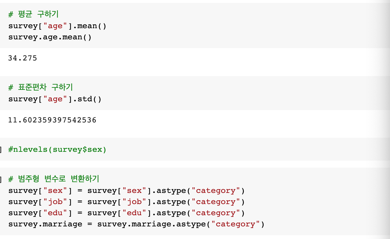
# 평균 구하기
survey["age"].mean()
survey.age.mean()
# 표준편차 구하기
survey["age"].std()
# nlevels(survey$sex)
# 범주형 변수로 변환하기
survey["sex"] = survey["sex"].astype("category")
survey["job"] = survey["job"].astype("category")
survey["edu"] = survey["edu"].astype("category")
survey.marriage = survey.marriage.astype("category")
#nlevels(survey$sex)
# 연속인 변수의 기술통계량 구하기
survey.iloc[:, 1:].describe() # 1 다음부터 전체를 사용
agestat_by_sex = survey.groupby("sex")["age"].describe()
agestat_by_sex
agestat_by_sex["mean"] # 표준편차 : std
# (sex, marriage)를 그룹으로 age의 기술통계량 구하기
agestat_by_sex_marriage = survey.groupby(["sex","marriage"])["age"].describe()
agestat_by_sex_marriage
agestat_by_sex_marriage["mean"] # 표준편차 : std
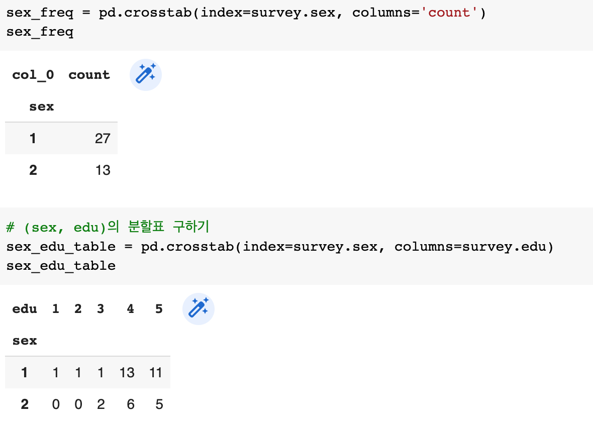
sex_freq = pd.crosstab(index=survey.sex, columns='count')
sex_freq
# (sex, edu)의 분할표 구하기
sex_edu_table = pd.crosstab(index=survey.sex, columns=survey.edu)
sex_edu_table
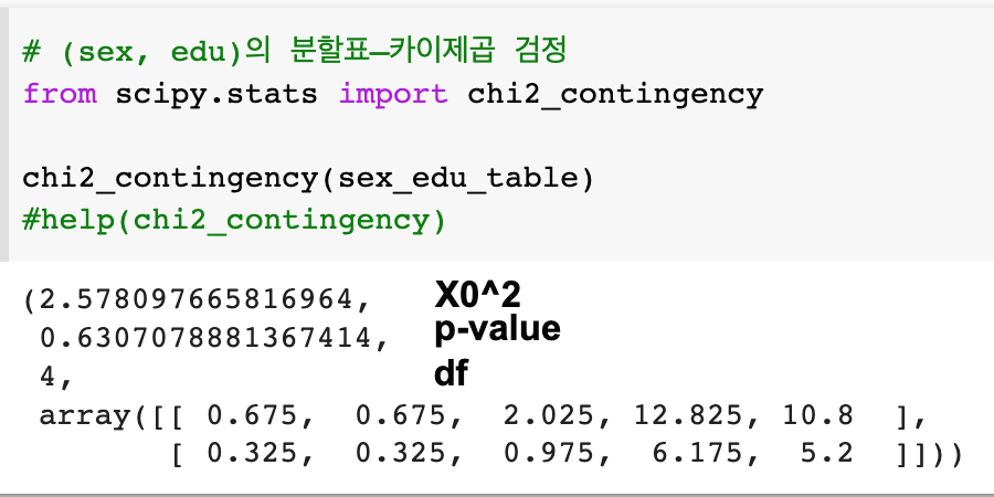
# (sex, edu)의 분할표–카이제곱 검정
from scipy.stats import chi2_contingency
chi2_contingency(sex_edu_table)
help(chi2_contingency)


반응형
'Data Science > Multivariate Analysis' 카테고리의 다른 글
| [Multivariate Analysis] Principal Component Analysis(PCA) 주성분분석 (0) | 2022.03.18 |
|---|---|
| [Mulivariate Analysis] eigenvalue(고유값)과 eigenvector(고유벡터) (0) | 2022.03.18 |
| [Multivariate Analysis] 다차원 통계그래프 (0) | 2022.03.13 |
| [Multivariate Analysis] 이변량 통계그래프 (0) | 2022.03.13 |
| [Multivariate Analysis] 단변량 통계그래프 (0) | 2022.03.13 |


댓글